Pearson Edexcel · A-Level · Mathematics
Course version: 9MA0 · Version from Mar 2026
Interpret the solution of a differential equation in the context of solving a problem, including identifying limitations of the solution; includes links to kinematics
Specification point 8.8 turns differential equations into real-world modelling: candidates must solve a rate equation, select the correct solution from initial conditions, and explain what the result means. The highest-value marks usually come at the end, when you interpret units, limits and model limitations rather than stopping at algebra.
- 10 min read
- 3 worked examples
- 5 practice questions
- 8 key terms
Check what you remember
Read the wording for your board, then hide it and explain Differential equation in your own words. Rough notes are fine. This is a self-check, with no mark or grade.
Reference: Pearson Edexcel
An equation relating a variable to one or more of its rates of change.
Study Notes

Overview
Pearson Edexcel A-Level Mathematics specification point 8.8 is where differential equations become modelling questions rather than a routine integration exercise. You must solve a first-order separable differential equation, select the correct particular solution using initial data, then explain what the result means in the situation. The specification explicitly requires you to consider validity for large values and connects the topic to kinematics. In an exam, a model may describe a leaking tank, a growing population, a balloon, or a particle whose speed changes with time.
Candidates often gain early method marks for correct separation and integration, then lose the final marks by treating the answer as an isolated formula. A complete response gives the numerical result with units, identifies its physical meaning, checks the permitted domain, and explains a realistic limitation. Typical command words are solve, show that, hence find, interpret, state, and suggest a limitation. Read the context before starting the calculus: it tells you which variable is time, which quantity changes, and what a sensible answer can look like.
Key Concepts
1. A differential equation is a rate statement in disguise
A differential equation relates a quantity to the rate at which it changes. If the depth of water is (H) metres and time is (t) hours, then (\frac{dH}{dt}) has units of metres per hour. A negative value means the depth is falling, while a positive value means it is rising. That sign must agree with the words in the question. For motion in a straight line, (\frac{dr}{dt}=v) and (\frac{dv}{dt}=a), so calculus translates directly into velocity and acceleration.
Before manipulating an equation, write a short variable key in the margin: (t\geq0), then identify the physical restrictions. Time after an event begins is normally non-negative. A radius, mass, depth, concentration, and speed cannot be negative. Displacement and velocity can be negative because they include direction. This is why a negative root may be algebraically possible but physically invalid.
Examiner habit: a contextual answer is stronger when it names the quantity and unit. Write “the water depth is 1.20 m” rather than “1.2”. Credit is given for a conclusion that fits the situation, not just calculator output.
2. Solve the mathematics, then select the model
For a separable equation, rearrange so that all terms involving the dependent variable and its differential are together. Then integrate each side. Include the constant of integration: without it, there is no family of solutions and the initial condition cannot select the required model.
For example, if (\frac{dH}{dt}=-0.10e^{-0.25t}), then
[
H=\int -0.10e^{-0.25t},dt=0.4e^{-0.25t}+C.
]
If (H=1.6) when (t=0), substitution gives (1.6=0.4+C), so (C=1.2). The particular solution is therefore (H=0.4e^{-0.25t}+1.2). The constant is not merely an algebraic leftover: it positions the curve so that it passes through the real starting condition.
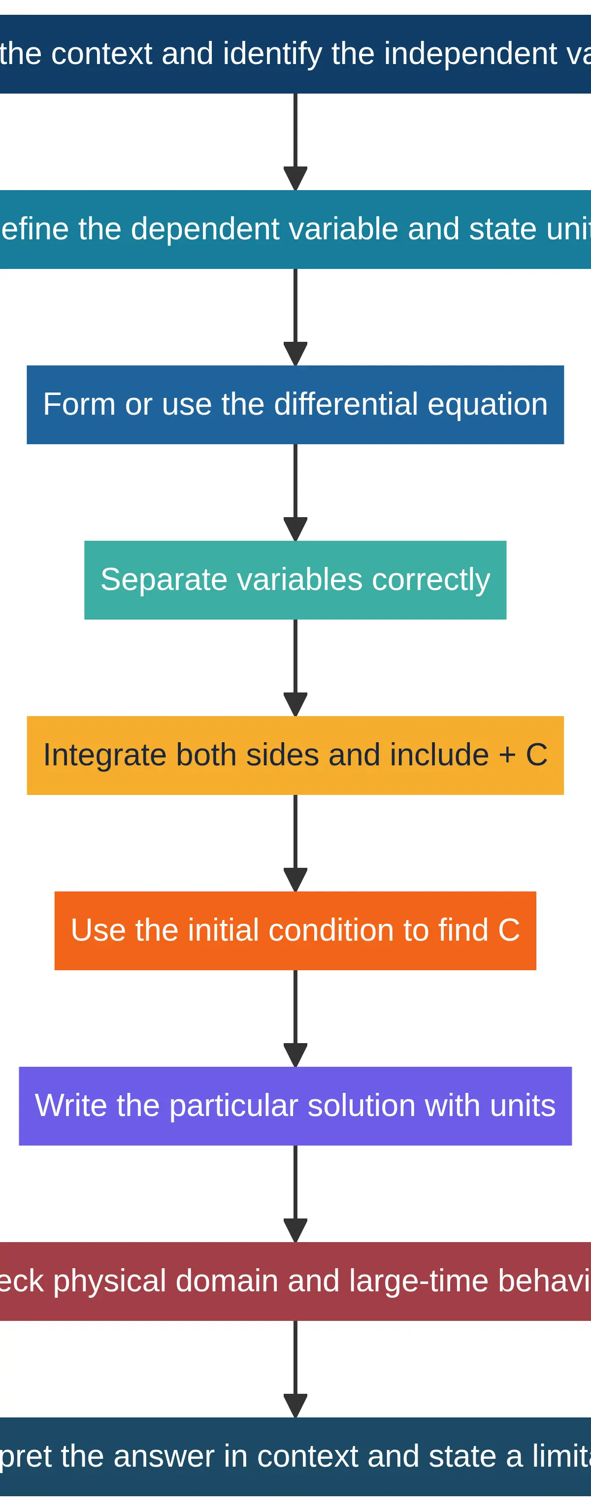
Memory hook: S-I-C-C. Separate, Integrate, use the Condition, then return to the Context. The final C earns the interpretation and limitation marks that candidates often miss.
3. Interpret large-time behaviour, not just a large calculator input
The wording “in the long term”, “as (t) becomes large”, “eventually”, or “find the limiting value” is a signal to analyse the behaviour of the expression. For (Ae^{-kt}+B), where (k>0), the exponential term tends to zero as (t\to\infty). Therefore the whole expression tends to (B).
In the water-depth example above, (H\to1.2) m. If water leaks through a hole in the side of the tank, 1.2 m can be interpreted as the height of the hole above the base. State that the depthapproaches 1.2 m. Do not say it reaches 1.2 m at a finite time unless your model proves that. An exponential tail approaches its limiting value indefinitely.
A good limitation connects the mathematics to an assumption. “The model is unrealistic” is too vague. Better answers are: “The model is likely valid only while the outflow law remains unchanged; in practice the hole may block,” or “The balloon model cannot hold indefinitely because a real balloon may burst and the inflation rate may change.” Marks are awarded for a precise model failure or neglected factor.
4. Kinematics is the same language with physical labels
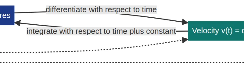
In one-dimensional motion, the chain is (r\rightarrow v\rightarrow a). Differentiate position to get velocity, and differentiate velocity to get acceleration. Integrate in the reverse direction, adding a constant each time. Initial position and initial velocity determine those constants. The units give a valuable check: (r) is measured in m, (v) in m s(^{-1}), and (a) in m s(^{-2}).

A velocity model such as (\frac{dv}{dt}=0.2(10-v)) says that acceleration is proportional to the gap between the current velocity and 10 m s(^{-1}). Its solution with (v(0)=2) is (v=10-8e^{-0.2t}). As (t\to\infty), (v\to10) m s(^{-1}), so 10 m s(^{-1}) is the modelled terminal velocity. If (v<10), acceleration is positive; as (v) nears 10, acceleration falls towards zero. This is an interpretation of the equation, not an extra calculation.
5. Domain, range and limitations are evidence, not decoration
Use the situation to decide where the formula applies. For a square-root model, ensure the expression inside the root is non-negative. For a logarithmic step, the argument must be positive. If solving gives negative time after a process starts, reject it with a brief contextual reason. If a model predicts negative water depth, a radius below zero, or unlimited physical growth, the formula has been used outside its useful range.
Ask four reality-check questions before you finish: What does the number represent? Are the units correct? Is the input in the physical domain? Does the large-time prediction make sense? A model can be mathematically correct and physically limited at the same time. This distinction is central to 8.8.
6. Build an examiner-readable conclusion
The last two lines of a modelling solution should read like a conclusion, not a calculation dump. A safe structure is: “When (t=\ldots), (H=\ldots) m; therefore the [named quantity] is [value] [unit].” If a limit is required, write “As (t\to\infty), (e^{-kt}\to0), so (H\to B) m. Therefore the model predicts that [contextual explanation].” This turns the mathematics into a marked answer.
For an evaluation mark, attach one precise condition: “This prediction is reliable only while ...”. Do not introduce a limitation that contradicts the question data. For example, a leaking-tank conclusion can question whether the outlet remains unobstructed, but it should not claim that time is negative. This disciplined ending also makes it easy for an examiner to award the final accuracy, interpretation and modelling marks separately.
Mathematical Relationships
| Relationship | Status | Meaning and use |
|---|---|---|
| (\frac{dy}{dx}=f(x)\Rightarrow y=\int f(x),dx+C) | Must memorise | Integration reverses a rate. Include (+C) for an indefinite integral. |
| (\int e^{kx},dx=\frac{1}{k}e^{kx}+C) | Must memorise | Use when integrating exponential rate models. Check the chain factor (k). |
| (\frac{dr}{dt}=v), (\frac{dv}{dt}=a) | Must memorise | Links calculus to motion in a straight line. |
| (v=u+at), (s=ut+\frac12at^2), (v^2=u^2+2as) | Given in Pearson formula booklet | Use only for constant acceleration. A differential-equation model may describe variable acceleration instead. |
A graph of (Ae^{-kt}+B) with (A,k>0) falls towards the horizontal asymptote (y=B). Label the asymptote and interpret it in context. For a velocity-time graph, the gradient is acceleration and the signed area is displacement. If a graph crosses the time axis, velocity changes sign, so the particle changes direction. Speed is (|v|), never negative.
Practical Applications
Differential-equation models are compact descriptions of changing systems. A tank model can describe a changing liquid depth. A resistance model can describe a vehicle approaching terminal velocity. A growth model can describe a population approaching an equilibrium. In each case, initial data fixes one specific curve and the long-term limit predicts an equilibrium or asymptote.
There is no required practical for this A-Level Mathematics specification point. Treat the “practical” skill as model validation: compare a prediction with a measured or stated value, identify the interval over which the assumptions are credible, and explain one reason why conditions may change. Keep units consistent. Common conversions are (1\text{ m}=100\text{ cm}), (1\text{ h}=3600\text{ s}), and (1\text{ m s}^{-1}=3.6\text{ km h}^{-1}). Convert before substituting, not after finding a time from a formula.
Exam-Focused Method
For each mark, show one meaningful step. First define the variables and units if the context is complicated. Second, set up or use the differential equation and rearrange it accurately. Third, integrate and retain (+C). Fourth, substitute the initial condition and write the particular solution in the requested form. Finally, use the solution to answer the actual wording: a numerical value, a limit, an explanation, or a limitation.
If the command word is show that, keep exact values and make the target expression visible. If it is hence, carry forward the model you have just found. If it is interpret, use a sentence containing the quantity, unit, and real-world meaning. If it is suggest a limitation, name a specific assumption that may fail. About one minute per mark is a sensible guide, although a six-mark modelling question may take six to seven minutes because contextual checking is part of the solution.
Cover and Recall
Cover the formula and say the S-I-C-C sequence aloud. Then explain why (+C) is necessary. Finally, look at any exponential solution and state its limiting value before you calculate anything. Retrieval is more valuable here than re-reading a model answer: it trains you to see both the calculus layer and the reality-check layer under exam pressure.
Visual Resources
2 diagrams and illustrations
Interactive Diagrams
2 interactive diagrams to visualise key concepts
Conceptual Flow Outline
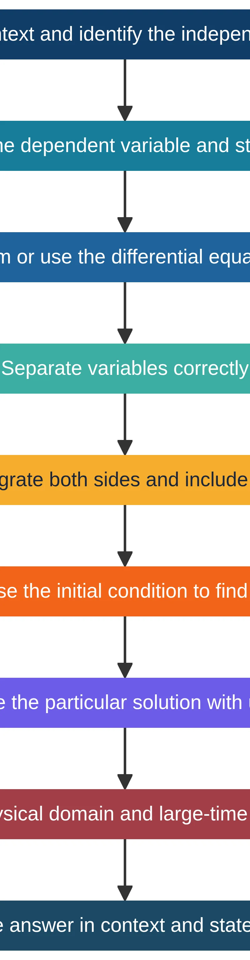
The S-I-C-C modelling workflow: calculus earns method marks, while interpretation and limitations complete the response.
Conceptual Flow Outline
The calculus links in straight-line kinematics: differentiate from position to acceleration and integrate back using initial conditions.
Worked Examples
3 worked examples — open one to explore the question and available guidance.
Practice Questions
Try the question, then reveal an answer plan or example response
The temperature T °C of a liquid satisfies dT/dt=-0.4T, where t is in minutes and T(0)=30. Find T in terms of t and state the limiting temperature.
Hint: Separate T from t, then use the initial condition after integrating.
The depth H m of water in a container satisfies dH/dt=-0.15e^{-0.3t}. Given H(0)=2.3, find H in terms of t and the long-term depth.
Hint: Integrating -0.15e^{-0.3t} gives +0.5e^{-0.3t}.
A particle has velocity v m s^-1 satisfying dv/dt=-0.2v and v(0)=12. Find the time when v=3. Interpret why this time is valid.
Hint: Your particular solution should be v=12e^{-0.2t}.
A spherical balloon has radius r cm modelled by dr/dt=3.6/√r, with r(0)=9. Find r(5) and state one limitation of using the model at very large times.
Hint: Multiply by √r before integrating, then use r^(3/2).
A vehicle’s speed v m s^-1 satisfies dv/dt=0.2(10-v), with v(0)=2. Show that v=10-8e^{-0.2t}. Hence explain the long-term motion and state one modelling assumption.
Hint: Use u=10-v after separating variables, or recognise a shifted exponential model.
Exam technique
How to turn what you know into marks
How to approach the question
Underline the changing quantity, independent variable, units and any initial condition. Apply S-I-C-C. Keep working exact until the required final accuracy. Before answering, check the physical domain and whether a limit is being requested.
How to structure your answer
For 1-2 marks, state the result with unit and a precise context phrase. For 3-4 marks, show separation/integration, use the condition, then state the result. For 5-6 marks, add a limit calculation, contextual sentence and one assumption-linked limitation.
Timing
Approximately 1 minute per mark. Allow 6-7 minutes for a 6-mark modelling question because the interpretation and limitation are part of the answer.
Common pitfalls
- Omitting +C after an indefinite integration. Avoid this by writing +C before using any initial condition.
- Using a large arbitrary value of t instead of evaluating the long-term limit. Write t→∞ and identify the exponential term tending to zero.
- Calling a negative velocity ‘negative speed’. State that the particle moves in the negative direction; speed is the magnitude of velocity.
- Giving a vague limitation. State a concrete assumption that may fail, such as constant resistance, an unchanged outflow law, or unlimited resources.
What the command words want
- Hence
- Use the model or result from the preceding part, rather than restarting with a new approach.
- Calculate
- Show the formula or solved equation, substitute accurately, then round only as instructed.
- Interpret
- Write a full sentence that names the physical quantity, gives the unit and explains what the numerical or limiting value means.
- Show that
- Present a logical chain of working ending exactly in the given target form; do not round intermediate values.
- State/Give
- Provide the requested value or phrase directly, including a unit where relevant.
- Suggest a limitation
- Identify one stated or implied assumption and explain briefly how it could fail in the real situation.
Watch or listen (optional)
Test your understanding of Interpret the solution of a differential equation in the context of solving a problem, including identifying limitations of the solution; includes links to kinematics
Active recall beats re-reading. Take an instant quiz now to test what you’ve learned and lock it into long-term memory.
7 days Premium · Then the free plan continues · No card, no charge